Climate models got their fundamentals right

Everyone loves to hate climate models: climate deniers of course, but also the climate scientists who do not use these models — there are many, from observationalists to theoreticians. Even climate modelers love to put their models through harsh reality checks, and I confess to have indulged in that myself: about how models represent of sea-surface temperature variations in the tropical Pacific on various time scales (here, and here), or their ability to simulate the temperature evolution of the past millennium.   

There is nothing incongruous about that: climate models are the only physically-based tool to forecast the evolution of our planet over the next few centuries, our only crystal ball to peer into the future that awaits us if we do nothing — or too little — to curb greenhouse emissions. If we are going to trust them as our oracles, we had better make sure they get things right. That is especially true of climate variations prior to the instrumental record (around 1850), since they provide an independent test of the validity of the models’ physics and assumptions. 

In a new study in the Proceedings of the National Academy of Sciences, led by Feng Zhu, a third-year graduate student in my lab,  we evaluated how models fared at reproducing the spectrum of climate variability (particularly, its continuum)  over scales of 1 year to 20,000 years. To our surprise, we found that models of a range of complexity fared remarkably well for the global-mean temperature — much better than I had anticipated. This is tantalizing evidence that models contain the correct physics to represent this aspect of climate, with a big caveat: they can only do so if given the proper information (“initial and boundary conditions”). While the importance of boundary conditions has long been recognized, our study shakes up old paradigms in suggesting that the long memory of the ocean means that initial conditions are at least as important on these scales:  you can’t feed your model a wrong starting point and assume that fast dynamics make it forget all about it within a few years or decades. The inertia of the deep ocean means that you need to worry about this for hundreds — if not thousands — of years. This is mostly good news for our ability to predict the future (climate is predictable), but means that we need to do a lot more work to estimate the state of the deep ocean in a way that won’t screw up predictions. 

Why spectra?

Let us rewind a bit. The study originated 2 years ago in discussions with Nick McKay, Toby Ault, and Sylvia Dee, with the idea of doing a Model Intercomparison Project (a “MIP”, to be climate-hip) in the frequency domain. What is the frequency domain, you ask? You may think of it as a way to characterize the voices in the climate symphony. Your ear and your brain, in fact, do this all the time: you are accustomed to categorizing the sounds you hear in terms of pitch (“frequency”, in technical parlance) and have done it all your life without even thinking about it. You may even have interacted with a spectrum before:  if you have ever tweaked the equalizer on your stereo or iTunes, you understand that there is a different energy (loudness) associated with different frequencies (bass, medium, treble), and it sometimes need to be adjusted. The representation of this loudness as a function of frequency is a spectrum. Mathematically, it is a transformation of the waveform that measures how loud each frequency is, irrespective of when the sound happened (what scientists and engineers would call the phase). 

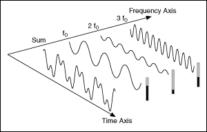
Fig 1: Time and Frequency domain. Credit: zone.ni.com

 

 

If you’re a more visual type, “spectrum” may evoke a rainbow to you, wherein natural light is decomposed into its elemental colors (the wavelengths of light waves). Wavelengths and frequency are inversely related (by, it turns out, the speed of light). 

Fig 2: A prism decomposing “white” light into its constituent colors, aka wavelengths. Credit: DKfindout

So, whether you think of it in terms of sound, sight, or any other signal, a spectrum is a mathematical decomposition of the periodic components of a  signal, and says how intense each harmonic/color is.

Are you still with us? Great, let’s move on to the continuum. 

Why the continuum?

A spectrum is made of various features, which all have their uses. First, the peaks, which are associated with pure harmonics, or tones. The sounds we hear are made of pure voices, with a very identifiable pitch; likewise, the colors we see are a blend of elemental colors.  In the climate realm, these tones and colors  would correspond to very regular oscillations, like the annual cycle, or orbital cycles. All of these show up as sharp peaks in a spectrum. Then there are voices that span many harmonics, like El Niño, with its irregular, 2-7yr recurrence time, showing up as a broad-band peak in a spectrum. Finally, there is all the rest: what we call the background, or the continuum. You can think of the continuum as joining the peaks together, and in many cases it is at least as important as the peaks.

Why do we care about the continuum? Well, many processes are not periodic. To give but one example, turbulence theories make prediction about the energy spectrum of velocity fluctuations in a fluid, characterized by “scaling” or “power law”  behavior of the continuum.  There are no peaks there, but the slope of the spectrum (the “spectral exponent”) is all the rage: its value is indicative of the types of energy cascades that are at play. Therefore, these slopes are very informative of the underlying dynamics.   Hence the interest, developed by many previous studies, in whether models can reproduce the observed continuum of climate variability: if they can, it means they correctly capture energy transfers between scales, and that is what scientists call a “big fucking deal” (BFD). 

Our contribution

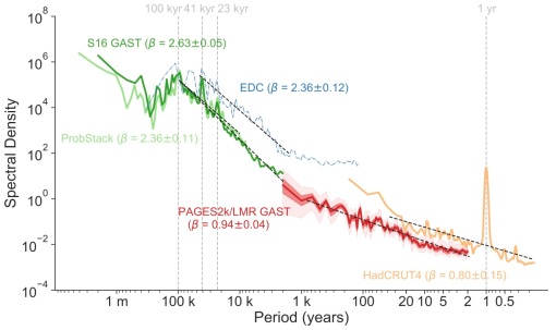
Fig 3: A spectral estimate of the global-average surface temperature variability using instrumental and paleoclimate datasets, as well as proxy-based reconstructions of surface temperature variability. See the paper for details.

One challenge in this is that we do not precisely know how climate varied in the past — we can only estimate it from the geologic record. Specifically, the data we rely on came from proxies, which are sparse, biased and noisy records of past climate variability. I was expecting to find all kinds of discrepancies between various proxies, and was surprised to find quite a bit of consistency in Fig 1. 

In fact, because we focused on global scales, the signal that emerges is quite clean: there are two distinct scaling regimes, with a kink around 1000 years. This result extends the pioneering findings of Huybers & Curry [2006], which were an inspiration for our study, as were follow-up by Laepple & Huybers [2013a,b, 2014].

It also leads to more questions:

– Why do the regimes have the slopes that they do?

– Why is the transition around 1,000 years?

– Can this be explained by a simple theory, based on fundamental principles?

This we do not know yet. What we did investigate was our motivating question: can climate models, from simple to complex, reproduce this two-regime affair? Why or why not?

What we found is that even simple models (“Earth System Models of Intermediate Complexity”) or a coarse-resolution Global Climate Model (GCM) like the one that generated TraCE-21k capture this feature surprisingly well (Fig 4).

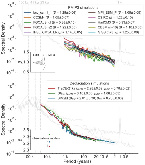
Fig 4: The power spectral density (PSD) of transient model simulations. In the upper panel, β is estimated over 2-500 yr. The inset plot compares distributions of the scaling exponents (estimated over 2-500 yr) of GAST in PAGES2k-based LMR vs the PMIP3 simulations. The inset plot compares the β values of the model simulations (red, green, and blue dots) and that of the observations (gray dots). The gray curves are identical as those in Fig. 1. See Zhu et al [2019] for details

The TraCE-21k experiments were designed to simulate the deglaciation (exit from the last Ice Age, 21,000 years ago), and they know nothing about what conventional wisdom says are the main drivers of climate variations over the past few millennia: explosive volcanism, variations in the Sun’s brightness, land-use changes, or, more recently, human activities, particularly greenhouse gas emissions. And yet, over the past millennium, these simple models capture a slope of -1, comparable to what we get from state-of-the-art climate reconstructions. Coincidence?

More advanced models from the PMIP3 project also get this, but for totally different reasons. Most PMIP3 models don’t appear to do anything over the past millennium, unless whacked by violent eruptions or ferocious emissions of greenhouse gases (a.k.a. “civilization”). If you leave these emissions out, in fact, the models show too weak a variability, and too flat a spectral slope.  How could that be, given that they are much more sophisticated models  than the ones used to simulate the deglaciation?

Does the ocean still remember the last Ice Age?

The answer comes down to what information was given to these models: you can have the most perfect model, but it will fail every time if you give it incorrect information. In the PMIP experimental protocol, the past1000 simulations are given a starting point that is in equilibrium with the conditions of 850 AD. That makes sense if you’re trying to isolate the impact of climate forcings (volcanoes, the Sun, humans) and how they perturb this equilibrium. But that implicitly assumes that there is such a thing as equilibrium. Arguably, there never is: the Earth’s orbital configuration is always changing, and if the climate system is always trying to catch up with it. Only a system with goldfish memory of its forcing can be said to be in equilibrium at any given time. So how long is the climate system’s memory? 

What TraCE and the simple EMICs show is that you can explain the slope of the continuum over the past millennium by climate’s slow adjustment to orbital forcing, or abrupt changes that happened over 10,000 years ago. This means that climate’s memory is in fact quite long. Where does it reside?  Three main contenders:

1. The deep ocean’s thermal and mechanical inertia
2. The marine carbon cycle
3. Continental Ice sheets

This is where we reach the limit of the experiments that were available to us: they did not have an interactive carbon cycle or ice sheets, so these effects had to be prescribed. However, even when all that is going on is the ocean and atmosphere adjusting to slowly-changing orbital conditions, we see a hint that the ocean carries that memory through the climate continuum, generating variability at timescales of decades to centuries, much shorter than the forcing itself. Though this current set of experiments cannot assess how that picture would change with interactive ice sheets and carbon cycle, it led to the following hypothesis (ECHOES): today’s climate variations at decadal to centennial scales are echoes of the last Ice Age; this variability arises because the climate system constantly seeks to adjust to ever-changing boundary conditions. 

If true, the ECHOES hypothesis would have a number of implications. The most obvious one is that global temperature is more predictable than has been supposed. The flipside is that this prediction requires giving models a rather accurate starting point. That is, model simulations starting in 1850 AD need to know about the state of the climate system at that time (particularly, the temperature distribution throughout the volume of the ocean), as this state encodes the accumulated memory of past forcings. Accurately estimating this state, even in the present day, is not trivial.

But first things first: is there any support for the ocean having such a long memory? Actually, there is: a recent paper by Gebbie & Huybers makes the point that today’s ocean is still adjusting to the Little Ice Age (around AD 1500-1800). Our results go a step further and suggest that the Little Ice Age, or the medieval warmth that preceded it, also lie on the continuum of climate variability. Though it is clear that they were influenced by short-term forcings, like the abrupt cooling due to large volcanic eruptions, part of these multi-century swings may simply be due to the ocean’s slow adjustment to orbital conditions. Fig 5 illustrates that idea. 

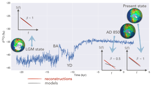
Fig 5: The impact of initial conditions on model simulations of the climate continuum. Models started with states in equilibrium with 850 AD show too flat a spectral slope unless whacked by the giant hammer of industrial greenhouse gas emissions. On the other hand, models initialized from a glacial state and adjusting to slowly-changing orbital conditions show a much steeper slope, comparable to reconstructions obtained from observations over the past 1000 years. This suggests that the continuum (some parts thereof, at least) is an echo of the deglaciation.

 

The ECHOES hypothesis is still only that: a hypothesis. It will take more work to test it in models and observations. But, if true, it would imply that even simple climate models correctly represent energy transfers between scales, i.e. that their physics are fundamentally sound. That’s a BFD if there ever was one in climate science. In the future, we would like to test this hypothesis with more complex models (with interactive carbon cycle and ice sheets), which will involve prodigious computational efforts.  If supported by observations, the ECHOES hypothesis will imply that to issue multi-century climate forecasts, one needs to initialize models from an estimate the ocean state prior to the instrumental era. This is a formidable challenge, but — trust us — we have ideas about that too.